femshop
Navier Stokes - 2D Driven lid
The Julia script: example-NS.jl
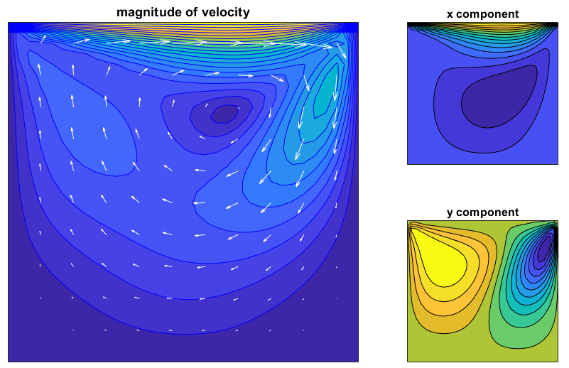
A 2D Navier Stokes simulation of a driven lid problem. This demonstrates the nonlinear solver capability, multiple variables, and parameter entities.
Begin by importing and using the Femshop module. Then initialize. The name here is only used when generating code files.
using Femshop
init_femshop("NS");
Then set up the configuration. This example simply sets dimensionality of the domain and polynomial order of the basis function space.
domain(2)                  	# dimension
functionSpace(order=4) 		# polynomial order
Use the built-in simple mesh generator to make the mesh and set up all node mappings.
mesh(QUADMESH, elsperdim=32, bids=4) # 32*32 elements, 4 separate boundary regions
Define the variable, test function, coefficient, and parameter symbols.
u = variable("u") 		# velocity x component
v = variable("v") 		# velocity y component
uold = variable("uold") # used for manually defining time derivatives
vold = variable("vold") #
p = variable("p") 		# pressure

du = variable("du") 	#
dv = variable("dv") 	# These three are being solved for
dp = variable("dp") 	# and are used by Newton's method.

testSymbol("w")

coefficient("mu", 0.01)
coefficient("dtc", dt)
coefficient("h", 1.0 / 32)
coefficient("coe1", 4.0)
coefficient("coe2", 6.0)

parameter("tauM", "1.0 ./ (coe1 ./ dtc ./ dtc+ (u*u+v*v) ./ h ./ h+coe2*mu*mu ./ h ./ h ./ h ./ h) .^ 0.5")
parameter("tauC", "0.1*h*h* ((u*u+v*v) ./ h ./ h+coe2*mu*mu ./ h ./ h ./ h ./ h) .^ 0.5")
Set up the time stepper and initial conditions. This example uses implicit Euler. Other explicit or implicit methods are available.
timeStepper(EULER_IMPLICIT)
dt = 0.05;
nsteps = 50;
setSteps(dt, nsteps) # use this to manually set the time steps

initial(u, "y > 0.99 ? 1 : 0")
initial(uold, "y > 0.99 ? 1 : 0")
initial(du, "0")
initial(v, "0")
initial(vold, "0")
initial(dv, "0")
initial(p, "0")
initial(dp, "0")
Convert the PDE into the weak form
The boundary conditions are specified.
boundary(du, 1, DIRICHLET, 0)
boundary(du, 2, DIRICHLET, 0)
boundary(du, 3, DIRICHLET, 0)
boundary(du, 4, DIRICHLET, 0)

boundary(dv, 1, DIRICHLET, 0)
boundary(dv, 2, DIRICHLET, 0)
boundary(dv, 3, DIRICHLET, 0)
boundary(dv, 4, DIRICHLET, 0)

boundary(dp, 1, NO_BC) # No boundary condition applied
boundary(dp, 2, NO_BC)
boundary(dp, 3, NO_BC)
boundary(dp, 4, NO_BC)
referencePoint(dp, [0,0], 0) # Pins a single Dirichlet point
Then write the weak form expression in the residual form. Finally, solve for u.
weakForm([du, dv, dp],
["w*(du ./ dtc + (u*deriv(du,1)+v*deriv(du,2) + deriv(u,2)*dv)) - deriv(w,1)*dp + mu*dot(grad(w), grad(du)) + tauM*(u*deriv(w,1)+v*deriv(w,2))*(du ./ dtc + (u*deriv(du,1)+v*deriv(du,2)) + deriv(dp,1)) - (w*((u-uold) ./ dtc + (u*deriv(u,1)+v*deriv(u,2))) - deriv(w,1)*p + mu*dot(grad(w), grad(u)) + tauM*(u*deriv(w,1)+v*deriv(w,2))*((u-uold) ./ dtc + (u*deriv(u,1)+v*deriv(u,2)) + deriv(p,1)))",
"w*(dv ./ dtc + (u*deriv(dv,1)+v*deriv(dv,2) + deriv(v,1)*du)) - deriv(w,2)*dp + mu*dot(grad(w), grad(dv)) + tauM*(u*deriv(w,1)+v*deriv(w,2))*(dv ./ dtc + (u*deriv(dv,1)+v*deriv(dv,2)) + deriv(dp,2)) - (w*((v-vold) ./ dtc + (u*deriv(v,1)+v*deriv(v,2))) - deriv(w,2)*p + mu*dot(grad(w), grad(v)) + tauM*(u*deriv(w,1)+v*deriv(w,2))*((v-vold) ./ dtc + (u*deriv(v,1)+v*deriv(v,2)) + deriv(p,2)))",
"w*(deriv(du,1)+deriv(dv,2)) + tauC*(deriv(w,1)*( du ./ dtc + (u*deriv(du,1)+v*deriv(du,2)) + deriv(dp,1) ) + deriv(w,2)*( dv ./ dtc + (u*deriv(dv,1)+v*deriv(dv,2)) + deriv(dp,2) )) - (w*(deriv(u,1)+deriv(v,2)) + tauC*(deriv(w,1)*( (u-uold) ./ dtc + (u*deriv(u,1)+v*deriv(u,2)) + deriv(p,1) ) + deriv(w,2)*( (v-vold) ./ dtc + (u*deriv(v,1)+v*deriv(v,2)) + deriv(p,2) )))"])

solve([du, dv, dp], [u, v, p, uold, vold], nonlinear=true);
End things with finalize_femshop() to finish up any generated files and the log.